In this earth climate system focus, Michael R. Gipp, Acting President from Marine Mining Corp, details the applications of discrete computation in paleoclimate systems
This paper introduces some concepts of the application of discrete computation in characterizing paleoclimatic systems. Such systems have chaotic inputs at different time and spatial scales. The methodology presented in this article was influenced by Crutchfield’s (1994) e-machine constructions, which were devised to characterize emergent behaviour in complex systems and appeared in Gipp (2022).
Earth’s climate system within a state space
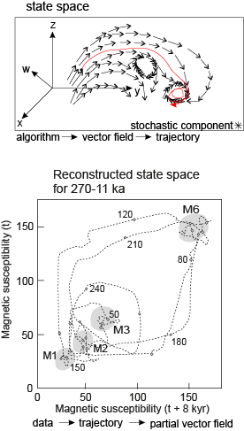
Earth’s climate system can be described by a series of equations within a state space defined by (presumably) real variables, such as atmospheric CO2 and global ice volume. The identity and the number of such variables are unknown, but the equations will populate state space with vectors which direct the evolution of the climate system (Figure 1).
From an initial point, the system will evolve along the vector field with a new state being defined by integrating the differential equations over infinitesimally small units of time (dt). The sequence of states typically generates a curved line called the trajectory of the system.
To obtain the vector field from observations, a reconstructed state space is created using state variables dependent on the set of observations. The reconstructed state-space trajectory will be topologically equivalent to that of the climate, and the direction of the vectors in the vicinity of the trajectory may be inferred.
In most cases, the vector field is relatively smooth in that there are only very small differences in direction and magnitude in vectors that are close to one another. In some small regions of state space, the vectors may all be directed to a point or possibly towards an ellipse –such features are called attractors.

Ergodic theory suggests that the number of attractors in the reconstructed state space will be the same in the climate system, provided the time is sufficient. There will be a one-to-one correspondence between attractors in the climate system and the reconstructed state space.
Figure 1 shows the last reconstructed state space of 260,000 years (ky) of the trajectory of the Himalayan paleomonsoon system (from Gipp, 2022). Although the last 650 ky of the system is characterized by seven attractors, the only attractors visited by the trajectory in this part of the record are designated M1, M2, M3, and M6.
Gipp (2022) proposed calling the individual observations ‘zero-order states’ and the attractors ‘first-order states’. The first-order states act as predictive and successor states – i.e., they have an order which can be determined using a discrete computation method already familiar to geologists – the Markov chain.
Discrete computation: The Markov chain
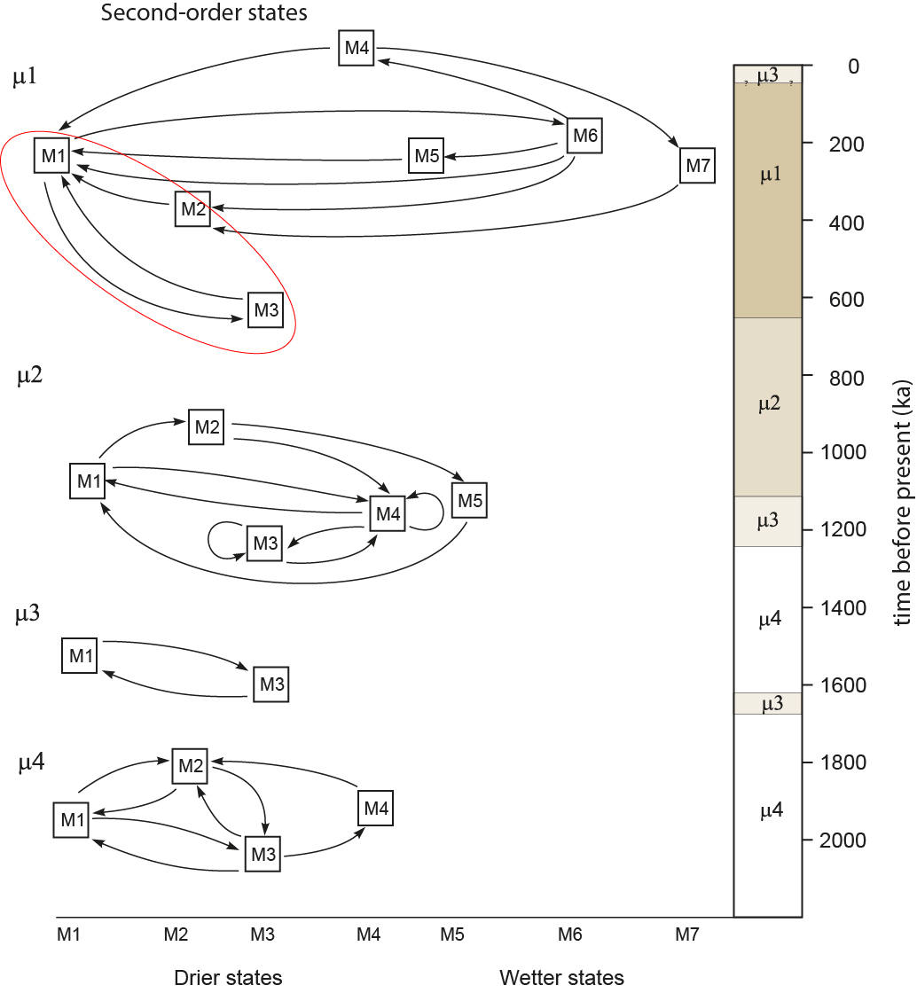
The Markov chain is found by identifying the string of attractors sampled by the trajectory as the system evolves through state space. The sequence of attractors is not necessarily the same each time the trajectory cycles through state space, nor are the same first-order states sampled every time. The Markov chain is built by considering the order of the first-order states, and noting which states follow. For instance, in Figure 2, during the last 630 ky, state M1 (a drier paleomonsoonal state) transitions only to M6 or M3.
The Markov chain represents another important property which will be representative of the natural algorithm. In Figure 2, we see that other time intervals in the Quaternary are characterized by Markov chains with different structures, and the succession of these can be described by another Markov chain. This, too, would be characteristic of the climate system.

The attractors, and the Markov chains formed from them, represent a hierarchy of chaotic dynamics operating in the earth system, which can be separated from one another through the use of the state space reconstruction and discrete computation.
References
- Crutchfield, J. P. (1994). The calculi of emergence: Computation, dynamics, and induction. Physica D, 75, 11- 54.
- Gipp, M. R. (2022). Extracting hierarchical dynamical structure from a multistable geological system – The Himalayan paleomonsoon, Paleoceanography and Paleoclimatology, 37(2), e2020PA004176. https://doi.org/10.1029/2020PA004176
Biography
Michael Gipp, currently acting president of Marine Mining Corp., is a geophysicist and sedimentologist. He has participated in nine voyages of oceanographic exploration and conducted fieldwork in the high Arctic, Arctic Scandinavia, Antarctica, West Africa, and many other places. He has taught at the University of Toronto, McMaster University, and the University of Waterloo.

This work is licensed under Creative Commons Attribution-NonCommercial-NoDerivatives 4.0 International.


